project 4
[Auto]stitching Photo Mosaics
Part 1: Shoot the Pictures
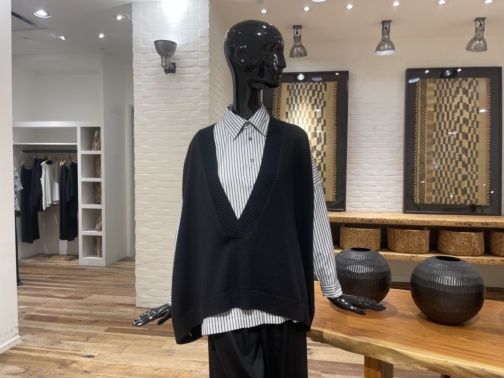
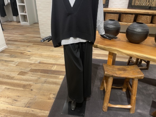
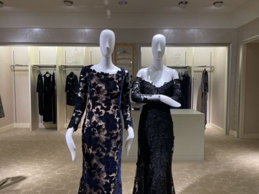
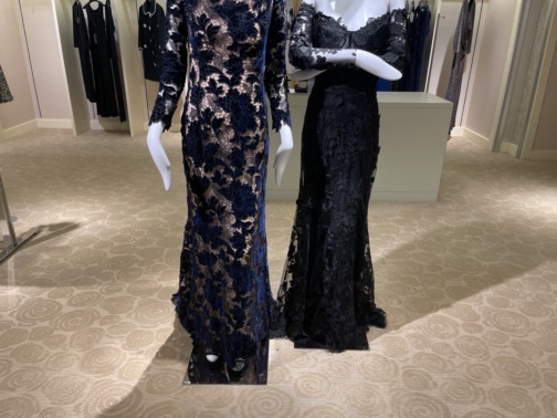
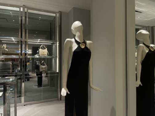
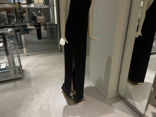
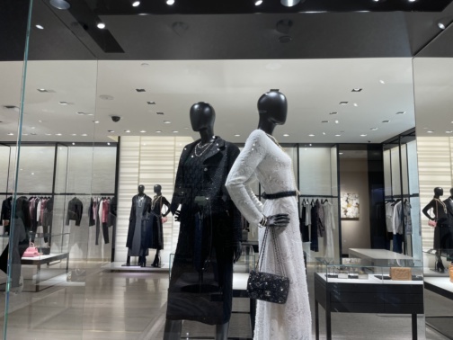
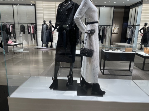
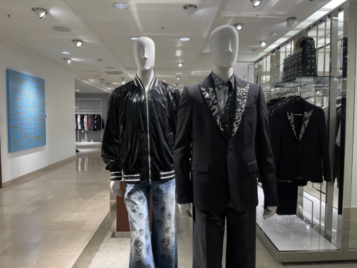
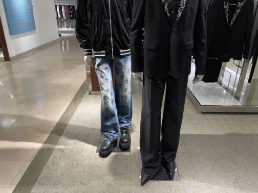
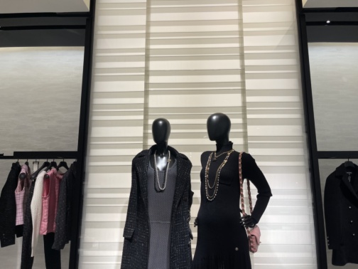
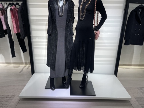
I went to a store and took pictures of mannequins wearing outfits I liked.
Part 2: Recover Homographies
Applying a homography reduces to a matrix multiplication \[ w \begin{bmatrix} x' \\ y' \\ 1 \end{bmatrix} = \begin{bmatrix} a & b & c \\ d & e & f \\ g & h & 1 \end{bmatrix} \begin{bmatrix} x \\ y \\ 1 \end{bmatrix} \] which can be rewritten as \[ \begin{aligned} wx' &= ax + by + c \\ wy' &= dx + ey + f \\ w &= gx + hy + 1 \end{aligned} \] \[ \implies \begin{aligned} (gx + hy + 1)x' &= ax + by + c \\ (gx + hy + 1)y' &= dx + ey + f \\ \end{aligned} \] \[ \implies \begin{aligned} x' &= ax + by + c - gxx'- hx'y\\ y' &= dx + ey + f - gxy'- hyy'\\ \end{aligned} \] But this is also just \[ \begin{bmatrix} x' \\ y' \end{bmatrix} = \begin{bmatrix} x & y & 1 & 0 & 0 & 0 & -xx' & -xy' \\ 0 & 0 & 0 & x & y & 1 & -yx' & -yy' \end{bmatrix} \begin{bmatrix} a \\ b \\ c \\ d \\ e \\ f \\g \\ h \end{bmatrix} \] so, given n correspondences, we can write this as a linear system \[ \begin{bmatrix} x_1 & y_1 & 1 & 0 & 0 & 0 & -x_1x_1' & -x_1y_1' \\ 0 & 0 & 0 & x_1 & y_1 & 1 & -y_1x_1' & -y_1y_1' \\ \vdots & \vdots & \vdots & \vdots & \vdots & \vdots & \vdots & \vdots \\ x_n & y_n & 1 & 0 & 0 & 0 & -x_nx_n' & -x_ny_n' \\ 0 & 0 & 0 & x_n & y_n & 1 & -y_nx_n' & -y_ny_n' \end{bmatrix} \begin{bmatrix} a \\ b \\ c \\ d \\ e \\ f \\g \\ h \end{bmatrix} = \begin{bmatrix} x_1' \\ y_1' \\ \vdots \\ x_n' \\ y_n' \end{bmatrix} \] and we can easily solve for the homography parameters using least squares.
Part 3: Warp the Images
To get the dimensions of the warped image, we can apply the homography matrix to the corners of the image and compute the bounding box of the warped image with these points (or we can skip this step altogether and just use the shape of thesource image for the warped image).
However, border points of the warped image can be negative, in which case we must calculate the offset to ensure that all indices in the warped image are non-negative.
Next, we calculate the height and width of the destination image, and use these dimensions to create indices for the warped image. We then apply the inverse offset to these indices (to align with the bounds of the warped image), and apply the inverse homography matrix to these translated indices. This will map the non-negative indices of the destination image to the source image.
Finally, we interpolate the pixels of the source image to the destination image
(I used scipy.interpolate.RectBivariateSpline),
and apply a mask to the destination image to remove the parts that are not in the source image.
Part 4: Image Rectification
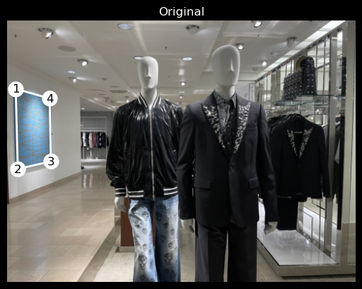
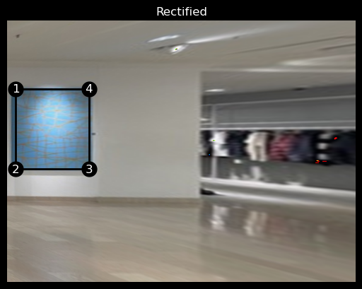
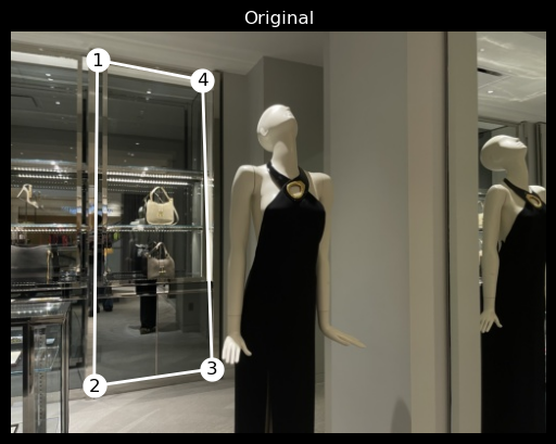
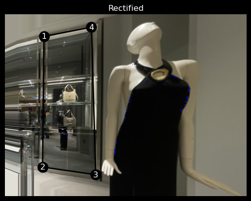
Here are some results I got from rectifying the images. [ note that I was able to avoid some inconveniences by using the shape of the source image for the warped image :D ].
Part 5: Blend The Images into a Mosaic
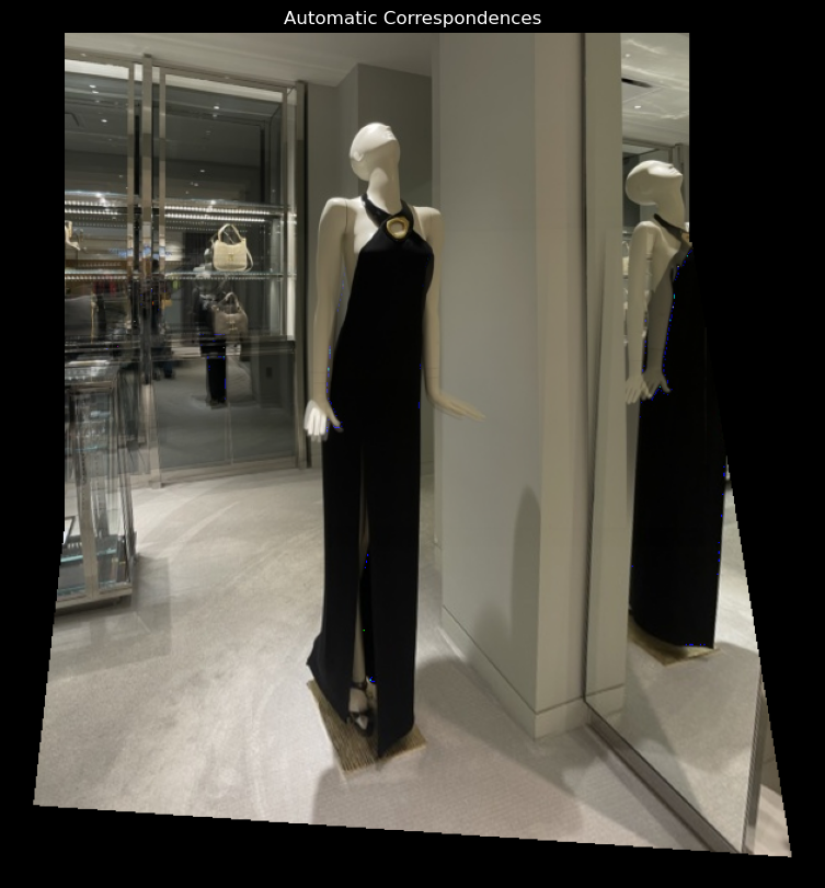
I was lazy ish and did not want to manually label correspondences between images. This led me to implement automatic non-maximal suppression, feature description extraction, and feature matching.
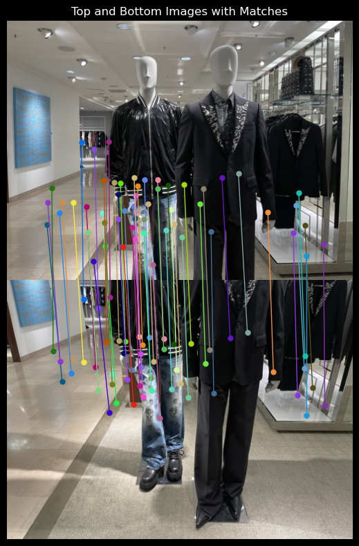
Here is an example of feature matching between two images.
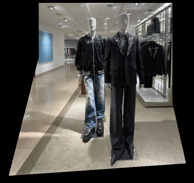
Using the matched features, I computed the homography between the base image (chosen to be the top), and the query image (the bottom).
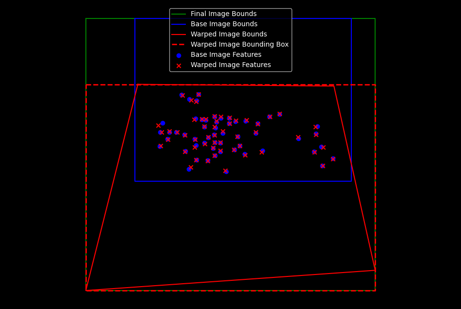
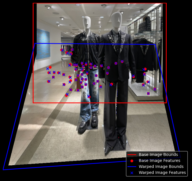
I warped the corners of the query image to the base image, then found the bounding box of the entire image after stitching. I computed the translation to apply to the final image to avoid negative indices.
This all boiled down to a mess of calling np.min and np.max on all sorts of corner points
and I really hope I never feel so confused with something so simple ever again.
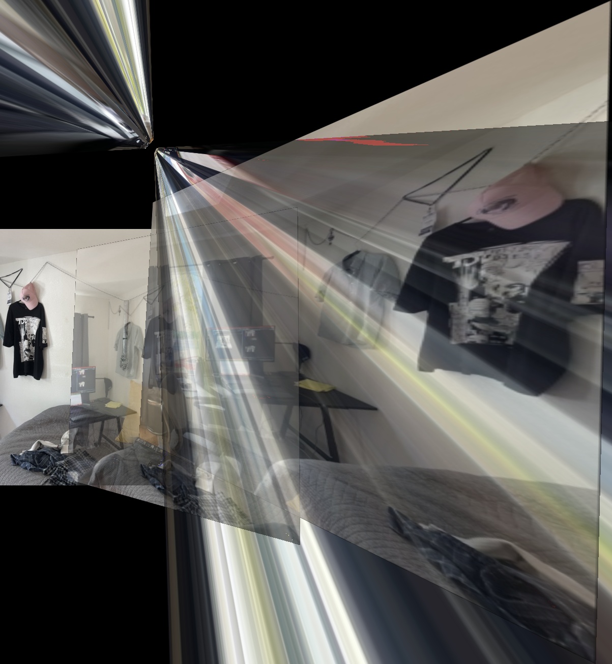
ok. cool.
I implemented blending with a two-level laplacian pyramid.
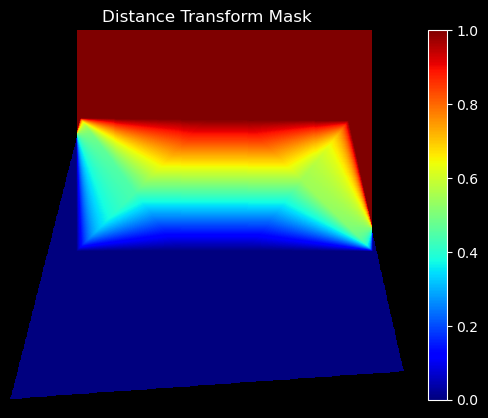
The mask was generated by taking the distance transform of the polygon made by the four corners of the images.
I used cv2.fillPoly to fill the polygon formed by vertices of img1 with 1,
then used cv2.distanceTransform to get the distance transform of the polygon.
I repeated this for img2,
and took the ratio of the distance transforms to get the blending mask.
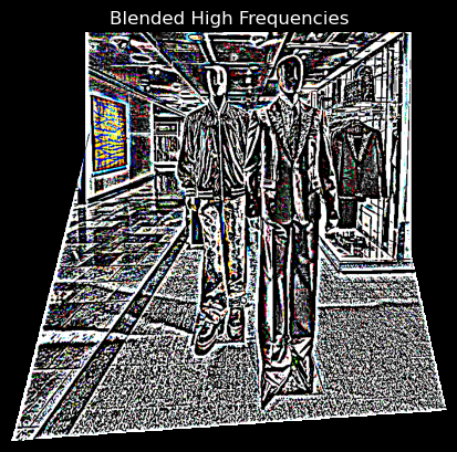
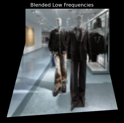
putting it all together
Part 5.X: Manual Correspondences
I thought I could get away with not manually labeling correspondences between images. I was wrong.

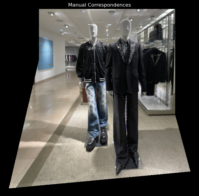
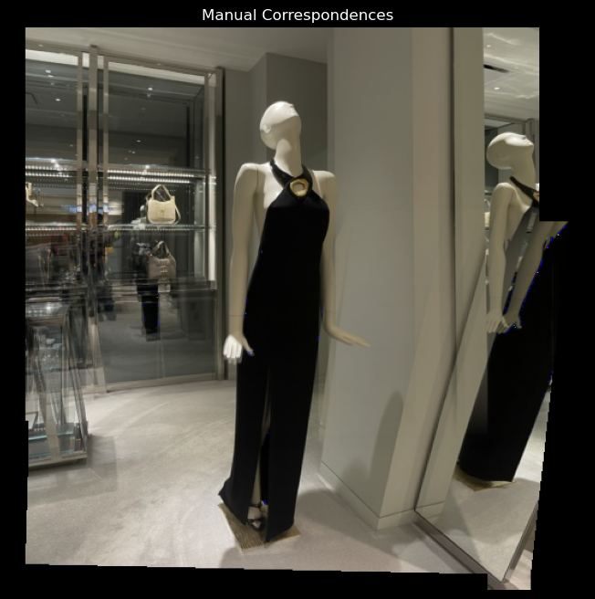
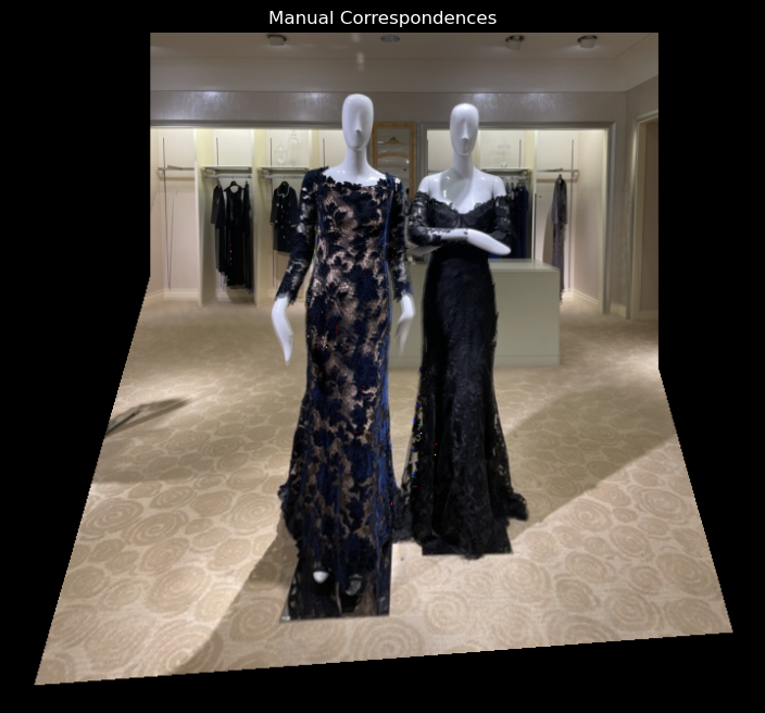
Here are some manually labeled correspondences and the mosaics they yielded.
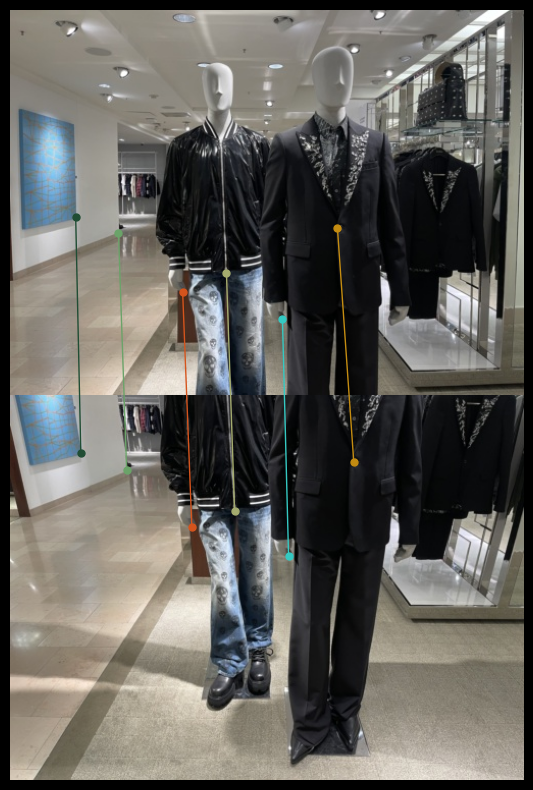
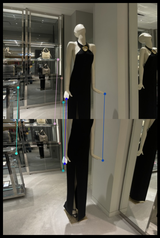
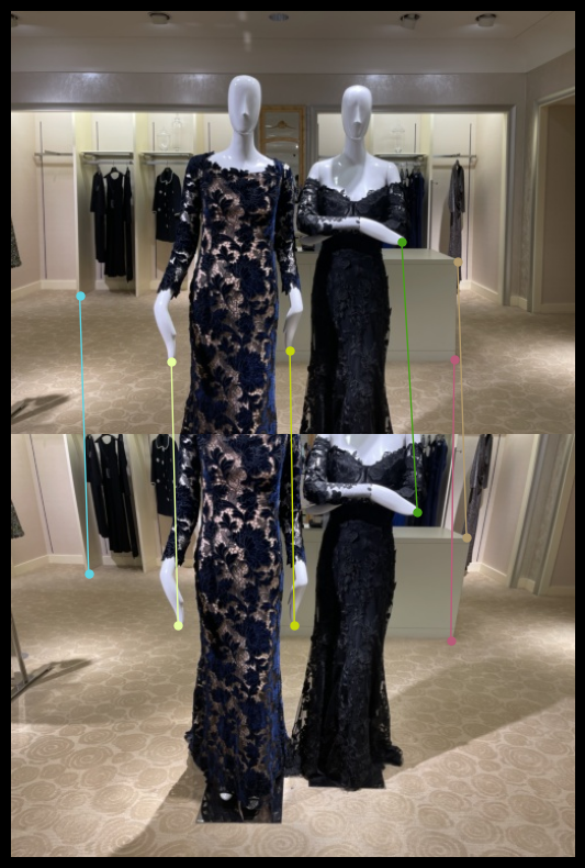
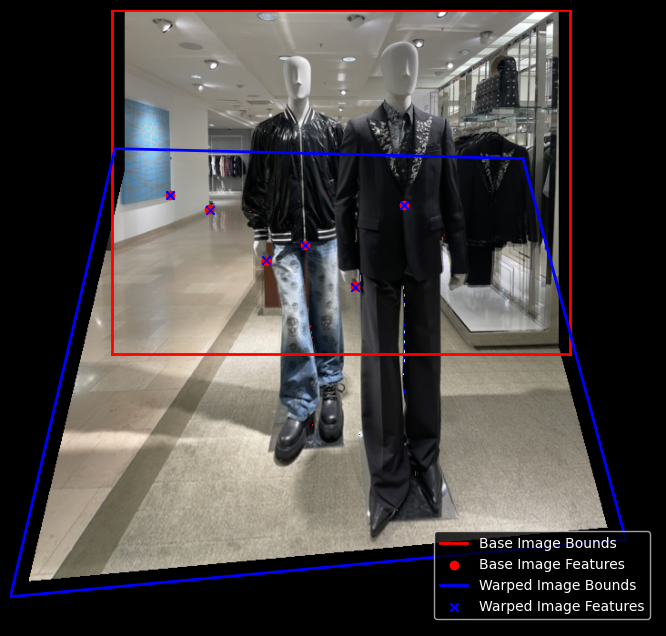
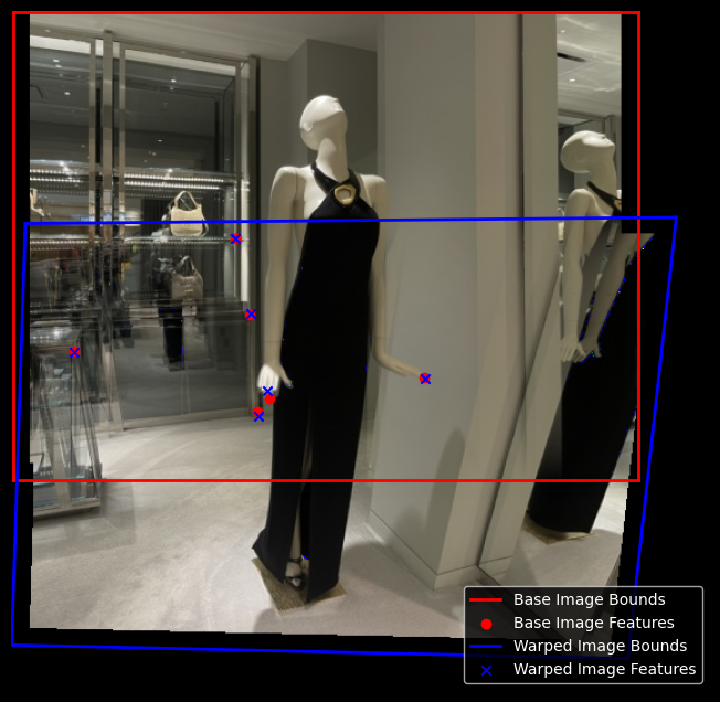
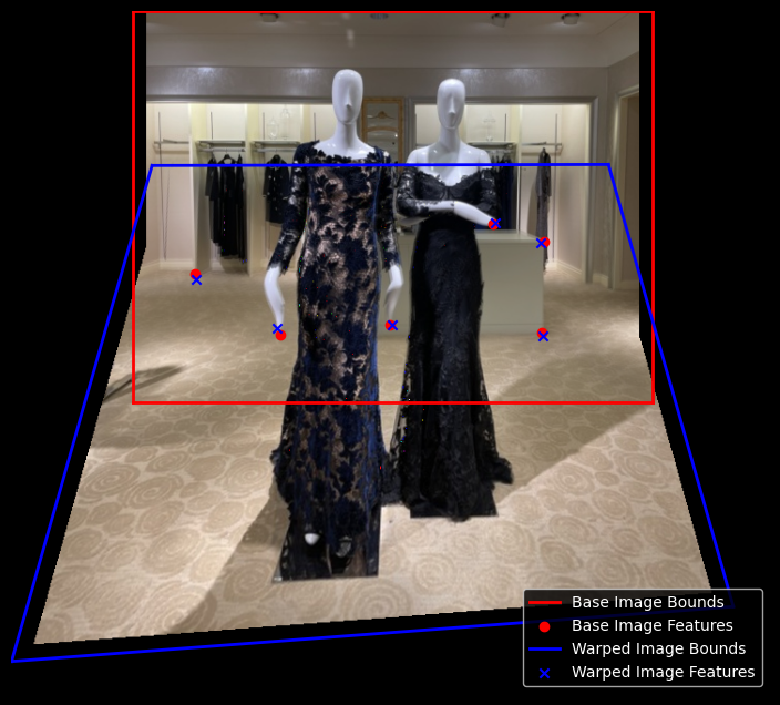
(after I mentioned that I implemented automatic correspondences, Prof. Efros told me that I should still do this step manually so I can understand the tediousness that motivates automating this process. It seems this fate was unavoidable)
Part 6: Detecting Corner Features in An Images
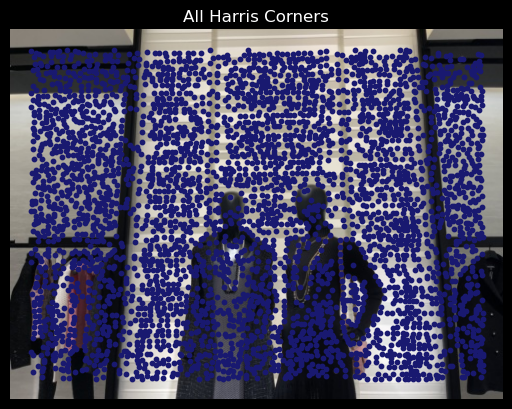
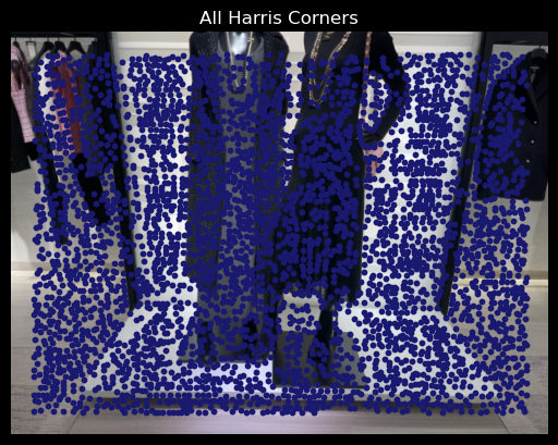
We use the Harris corner detector that was provided in the starter code (thank you!).
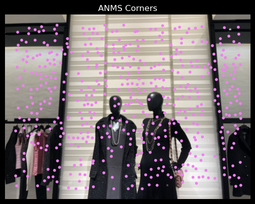
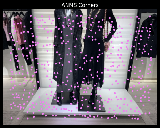
However, this is too many points! So we implement automatic non-maximal suppression to get the top corners. K-D Trees were particularly helpful. Here are the results of taking the top 500 corners.
Part 7: Extracting Feature Descriptors
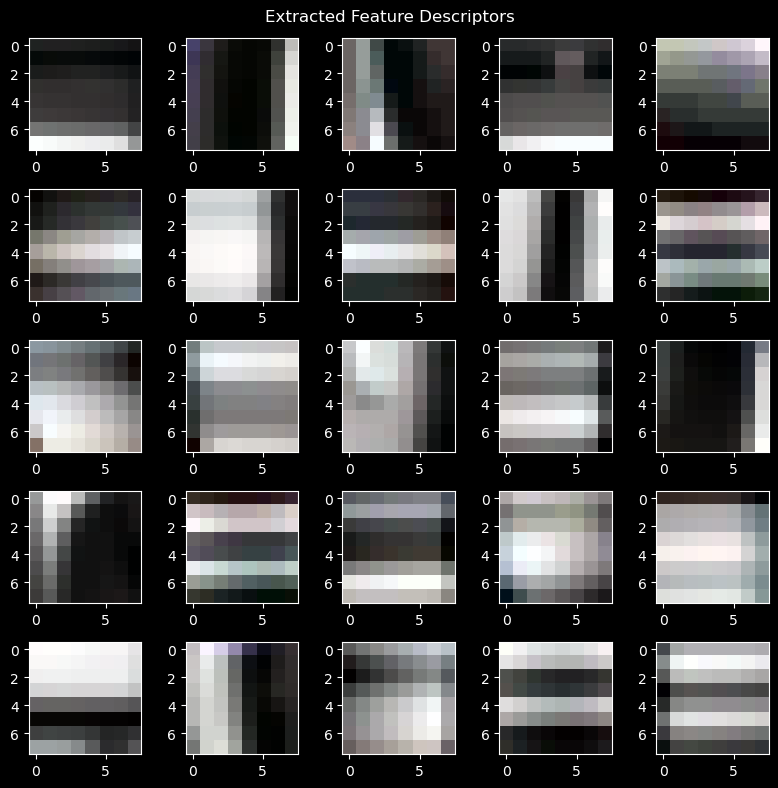
We take (8s)px x (8s)px patches centered around each corner returned by ANMS.
We then downsample each patch by taking every (s)th pixel and normalized each patch to have zero mean and unit variance.
Part 8: Matching Features Between Images
For every feature descriptor in image \(x\), we find the two most similar feature descriptors in image \(y\). In accordance to Lowe's test, we threshold the ratio \(r = \frac{err_{\text{1st match}}}{err_{\text{2nd match}}}\) as a test to remove bad matchings.
We cross-validate this by checking how many of the best matches from \(y\) are also the best matches for each feature descriptor in \(x\).
Part 9: RANSAC
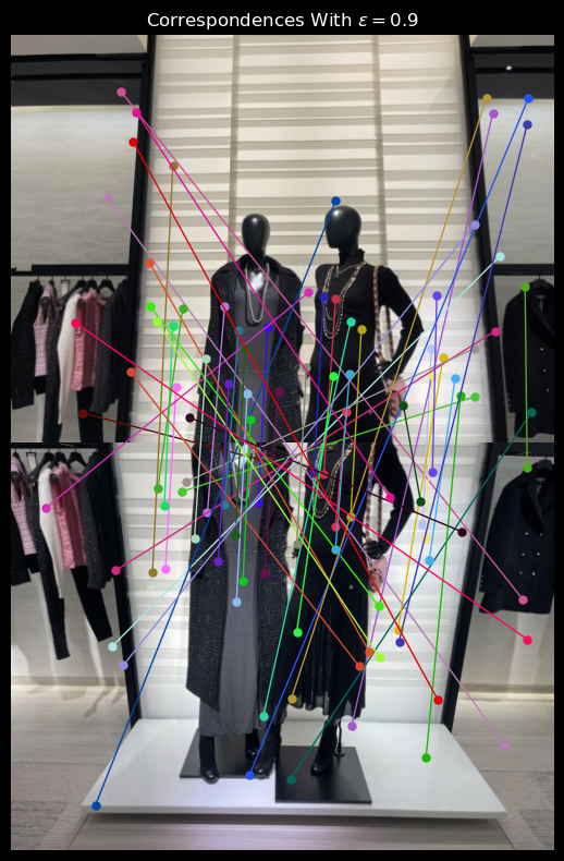
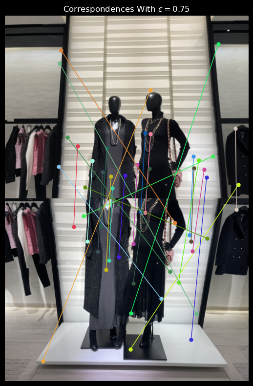
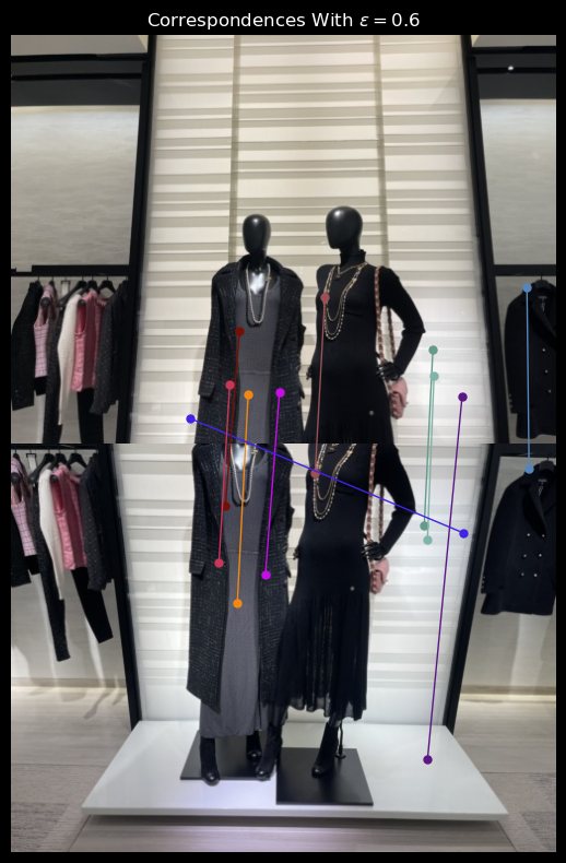
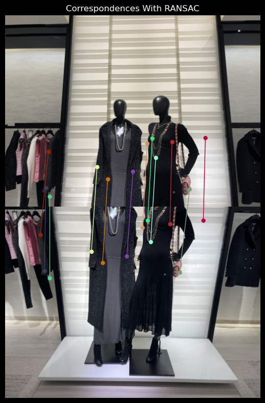
Some bad correspondences are unavoidable, so we use RANSAC to remove outliers.
The intuition behind RANSAC is to randomly sample a small number (4) of correspondences, compute the homography with this sample of source and destination points, apply the homography to all source points, and count how many warped source points are within some error threshold of their corresponding destination points. The correspondences within this threshold are inliers.
We repeat this process many times and keep the largest set of inliers as our correspondences.
Here are some results of RANSAC.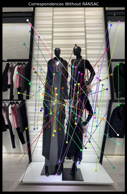
Part 10: More Mosaics
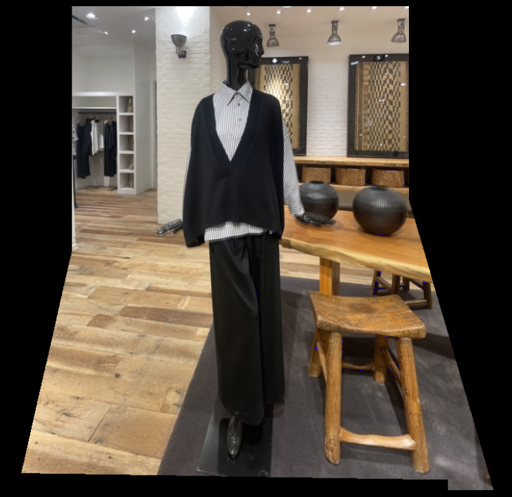
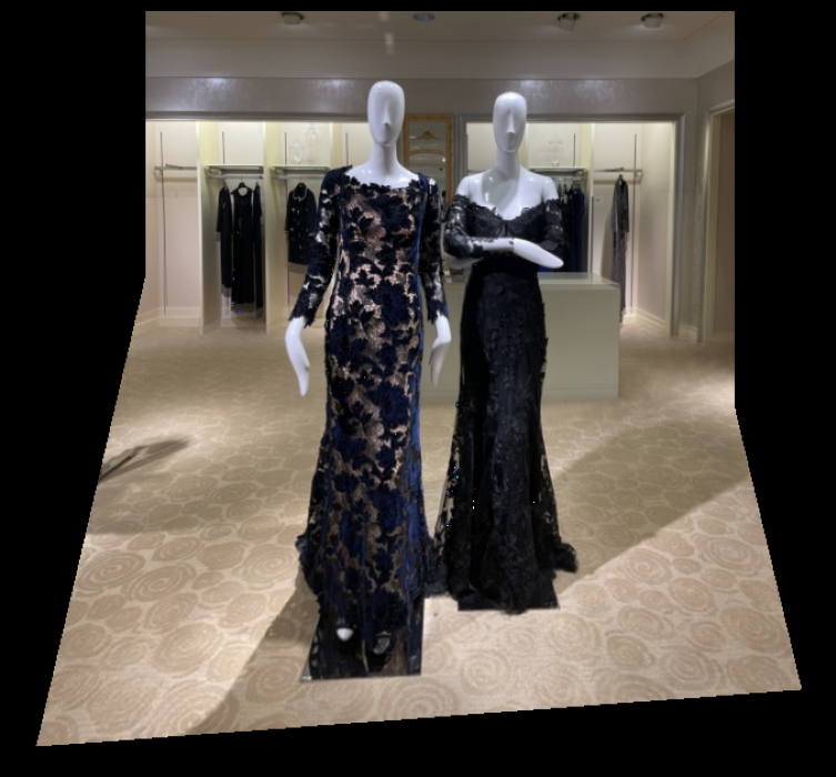
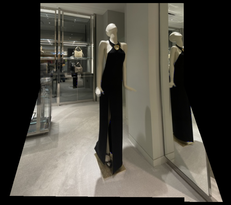
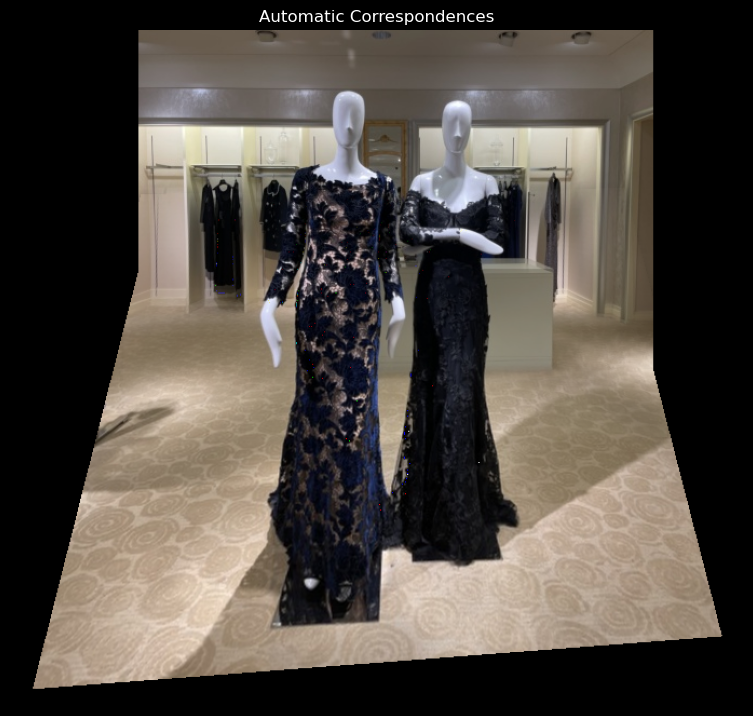
Here are all of the outfits I took pictures of, stitched together.
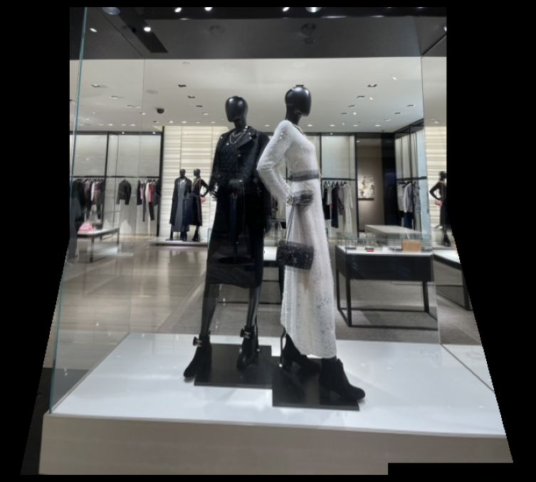
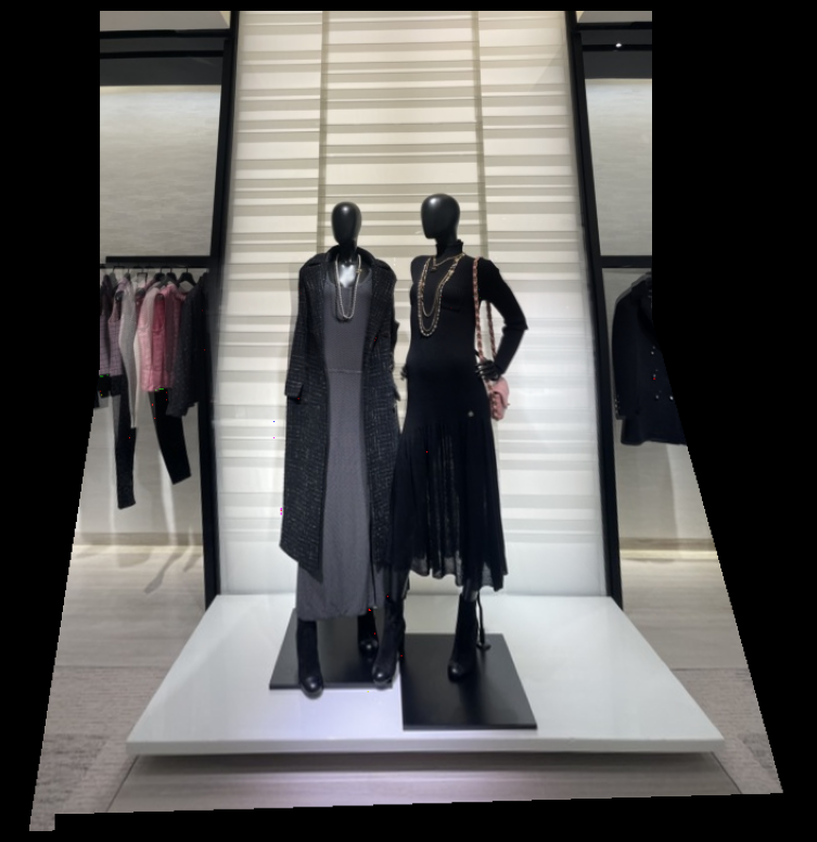

Here is a comparison of the mosaics from manual and automatic correspondences:

What have I learned?
I though it was interesting how the math underlying perspective warps is so simple. Considering how drastically the image changes after warping, I thought the whole procedure would be much more complicated.Ironically, the hardest part of this project was the blending step, which I had expected to be easy since I had done it for project 2. I did not expect to be so challenged by calculating the bounding box of the stitched image, the offset to avoid negative indices, and creating the blending mask.
I think the coolest and most important things I learned are:
- to not underestimate the simplicity of things that seem complex
- to not underestimate the complexity of things that seem simple
Extra: Ozan does not reinvent the wheel
The cv2.stitcher class is a wrapper for OpenCV's stitching functions.
I thought it would be fun to use this existing code, along with an HTML scipt I found online, to create a
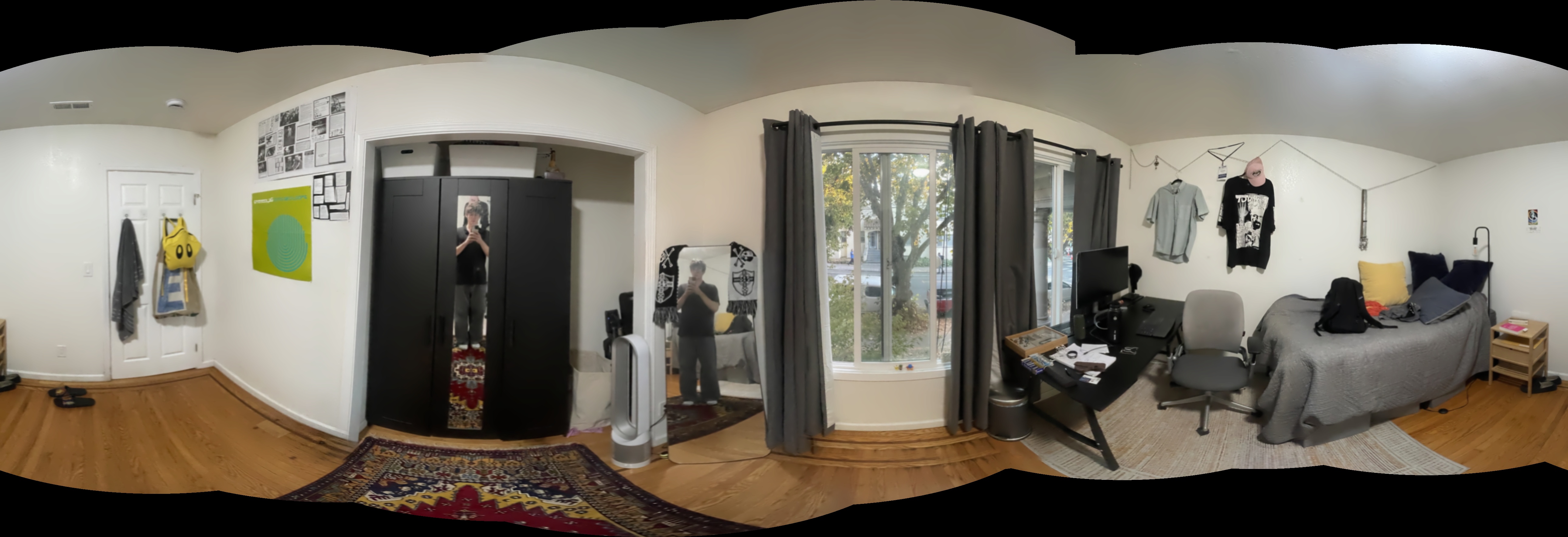
360° panorama viewer.
